Chalk X

Summary

• Part of a product manager’s job is to reduce the chance of an undesirable outcome, aka risk, of their product’s release.
• Humans are inherently bad at perceiving chance or changes in chance, which is one reason gambling is problematic. 
• Since humans are naturally unskilled in perceiving chance/risk, methodologies for calculating and visualizing are needed for better outcomes. 
• Using simplistic calculations, like averages, to mitigate risk can be dangerous because they hide outlier events and their impacts. Calculating all possible outcomes using simulations, visualizing, and facilitating conversation around them enables us to make better more transparent decisions. 

Chance is hard to feel:

Many people get nervous about flying. In recent years there have been 0 deaths for all US domestic flights. If you expand the scope to international aviation and go back several years the risk is about 1 in 2.067 million. The risk of a fatal crash in a motor vehicle is 1 out of 7,700 (based on US Department of Transportation data). These risks are so unbalanced that if we compare risk in terms of the miles traveled, a car trip of 12 miles is the same risk as any US domestic flight. Based on this data and where I live, it is 3 times more dangerous for me to go to the airport than to fly anywhere in the US. 

We don’t feel the difference in chance. Familiarity may be a greater factor in our feeling of ease than calculated outcomes since most of us drive more often than fly. Or it could be that we see plane crashes in the news but not car accidents. Ultimately humans are bad at dealing with unknowns and changes to chance and use informal heuristics to predict outcomes. Gambling is a good place where you can see this mismatch. When we play blackjack with friends we use one deck of cards but casinos use eight and constantly shuffle, which gives the casino a 41x increase in their chance to win. If there was ever a question if you were going to beat a Las Vegas casino look at the size of your house vs. the size of their hotel. They are winning most of the time.

Average at best (worse)

In flying or gambling, there is a range of possible outcomes. We are bad about guessing where we fall in that range. We think it is super likely the worse (flights) or best outcome (gambling) will occur. To mitigate this concern a common practice is to consider averages. The average outcome of a range is the most likely one, right?

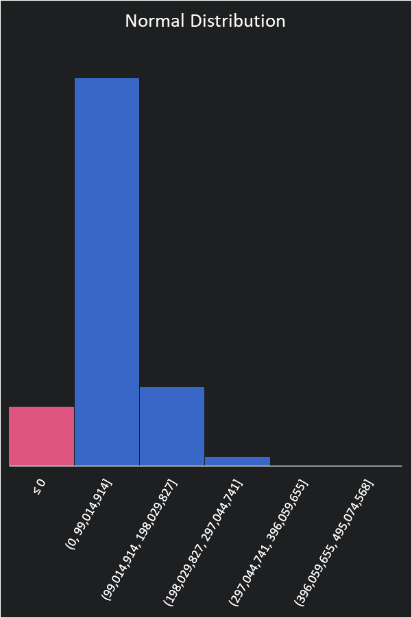
In Nassim Taleb’s book Fooled By Randomness, he asks us to imagine two countries, Mediocristan and Extremistan. In Mediocrastan most people are near the average height and weight and all make about the same amount of money. In Extremistan people are at the extremes in all things weight, height, and wealth. Meaning most live in extreme poverty but there are a few people with extreme wealth. Human traits exist within a relatively small distribution like height and weight. In a sampling of 1000 people if 2 people weigh 500 pounds, then that doesn’t change the average much. Averages in these narrow bands are mostly accurate in representing the whole. Below is a normal distribution of wealth, height, or weight of the people in the imaginary country of Mediocristan.

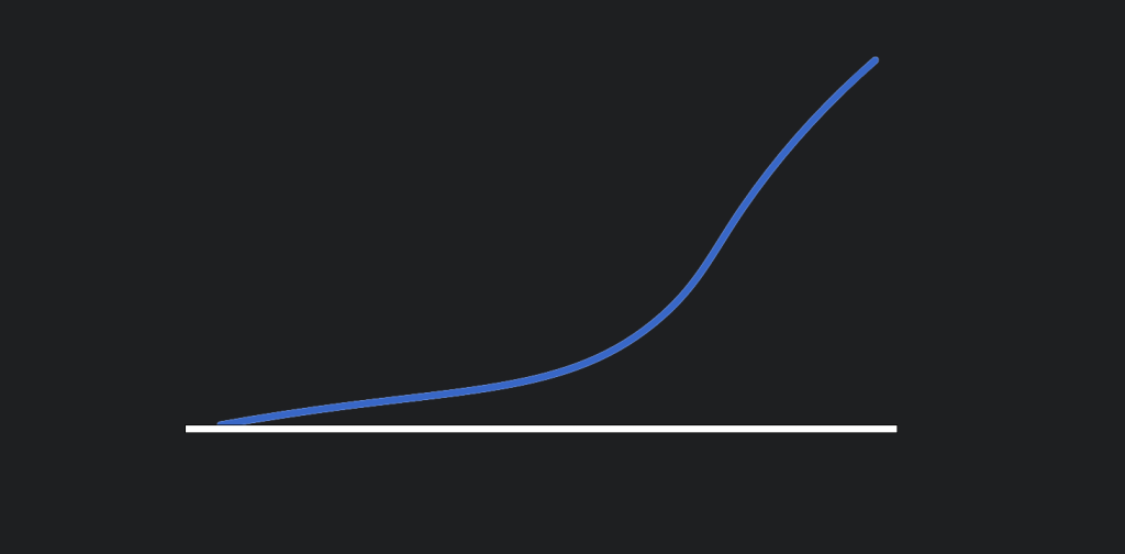
However, when it comes to wealth there can be a larger range. In Extremistan, you could have 999 people with a net worth of $1 but 1 person with a net worth of $100 billion.

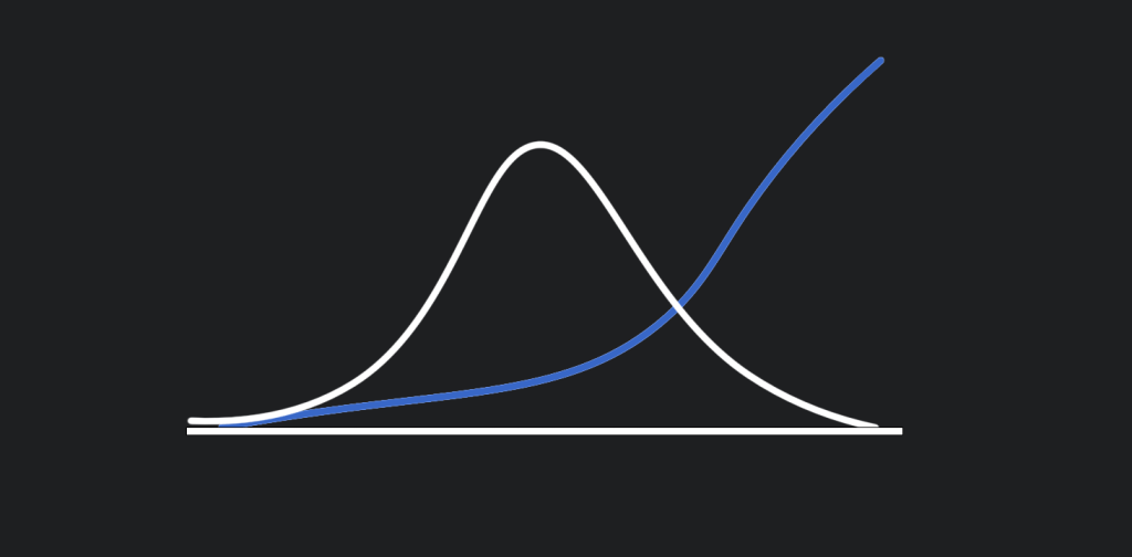
The average of these two societies is the same but the outcome for the individuals is wildly different. A single change to Extremistan, like one wealthy person leaving, can dramatically affect the whole. Now imagine making a product and trying to sell it to both countries because they have the same average income. Likely Mediocrastan will buy way more than the people in Extremistan where you may only sell your product to one person. These two curves have the same average:

High impacts for rare events

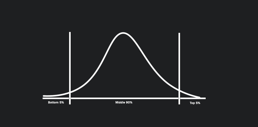
Consider the curves being not of a population but of possible outcomes. A rare outcome may have a huge impact and therefore should not be ignored. The easiest way to see the impact of extreme risk is from an example by Nassim Taleb, “If there is a 1% chance there is botulism in this glass of water would you drink it?” Most of us would say of course not, we’ll find something else to drink. But on average with every other glass of water, it is safe. Rare events sit on either end of a probability curve of possible outcomes. If the range is normally distributed the most likely outcome is somewhere in the middle. Even though the bottom 5% or top 5% outcomes happen rarely, we should care about them because of the impact. If there is a 5% chance there is poison in my glass of water, I’ll have something else.  If there is a 5% chance the product I’m working on will lose more money than the company is worth, then we should probably mitigate that or find something else to work on.

Additionally, not everything is always distributed normally. Extreme values could be more likely like in Extremistan. Since we don’t feel the changes in chance and we also don’t intuitively understand different distributions of outcomes, we need to calculate them. Our calculations can’t use averages, even though an average is easy to calculate because they obscure two things:

1. Non-normal distribution of a range.
2. High impact for rare events

Dealing with risk:

Knowing that we can’t intuit chance and that there are various kinds of distributions of possible outcomes, how can we calculate the chance of a combination of chances? Usually, a project is made up of multiple estimates like product development time is 2-8 weeks, possible product demand is 100-500 Units, or margins could be 30%-50%. These ranges interact with one another.

The temptation is to take the average of each of our ranges and add, multiply, subtract, divide, etc. the averages. Averages obfuscate the extremes and the impacts. We also don’t know which variable may influence potential negative outcomes the most.  Combining averages further obfuscates our risk conditions.

Luckily there is a way to simulate all possible outcomes and give us insight. One way to simulate multiple variables is by using a Monte Carlo simulator. Like a roulette wheel, a Monte Carlo simulator is a computer program that will randomly pick values in a range. Because we run this in a computer we can run this sampling thousands of times for the most probable values within a range.

For example, let’s assume for a given project we estimate that it takes between 1-10 weeks to get it done. If we roll truly randomly we we get each number as equally likely. However, 1 and 10 weeks are very unlikely. We will most likely get it done between 4-8 weeks. This is a normal distribution and we want to simulate this distribution. We will sample the most likely outcomes as well as edge cases but weighted toward the 4-8 range. This will help us simulate various scenarios with the right percentages. 

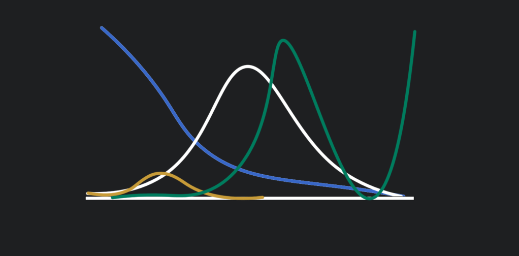
A robust simulator generates numbers based on each range’s specific possible distribution. Different distribution curves, like log rhythmic, can be used for ranges that are similar to Extremistan. For those that fall in the normal distribution curve, we can model them like the distribution of Mediocristan.

Additionally, we can add logic to our model with the interplay of variables, for example when we take 10 weeks or longer to develop or product we will miss a key trade show, and the chance of success is then 0. 

This is one of those things that is hard to discuss in the abstract, by completing a more complete scenario we can illustrate the building of a simulator.

Note: Most of what is used in this simulator example is based on methodologies from:

How to Measure Anything: Finding the Value of Intangibles in Business 3rd Edition
by Douglas W. Hubbard (Author)

Monte Carlo Simulator Scenario: 

Let’s assume our company has a new product opportunity. We are gathering our experts to estimate its potential success. For now, I will skip the risk discovery and estimation process, as that is a couple of articles in and of itself. 

We gather our key resources together to share our estimates and build our model. Our dev team thinks they can finish the project in 1-10 weeks depending on feature changes. Our current dev team costs around $1 million a week. In our tool, we label this range as Dev Costs. 

Our sales department is confident that if we are first to the market we can get $100 per unit. However, there is a risk it could be as low as $20 per unit if our competitors beat us to the market. We will label this range ASP for Average Sales Price. They have worked with marketing and user research and collectively they believe the demand should be between 100,000-700,000 units a month.

We talk to our manufacturing department and this totally new tooling for them. Their past margins have been around 50% but they warn each product could cost us up to 10% depending on the design. We will label this range as Margins. 

Manufacturing is pretty sure they can make 100,000 units a month and maybe up to 500,000 units. They indicate at the current facility size there is no chance they could make the 700,000 units a month even though that could be the demand. We will limit this range in our simulation from 100k-500k and call it Production Level (units per month). 

A simple calculation of midpoints would indicate a positive return on our investment of $53.5M. But is this the most likely outcome? Let’s build a Monte Carlo Simulator and see the possible financial outcomes. Each roll of the wheel creates 1 possible point on each of the ranges provided, put all the rolls together and we get 1 possible outcome for our new product. In Excel, it could look something like this for our annual return:

=(([@[Production Level (units per month)]]*12)*([@ASP]*[@Margins]))-[@[Dev Costs]]

Many possible numbers are in the above ranges, and initially, we assume a normal distribution for each. We will run the simulation 15k times. The higher the number of simulations the more consistent the results. Each outcome is put into a bucket. We want to highlight any number below 0 because in those outcomes we won’t be making a profit. The results of our first simulation look like this:

Based on our initial calculations we actually have a ~90.5% chance of making a profit. Only ~9.5% of our simulations have us losing money. This is good news but the first simulation isn’t complete.

The sales team mentioned they were not confident about the $100 price point. They are more confident that they could get around $35. For this, we will use a beta distribution. This will reflect the more likely ASP: 

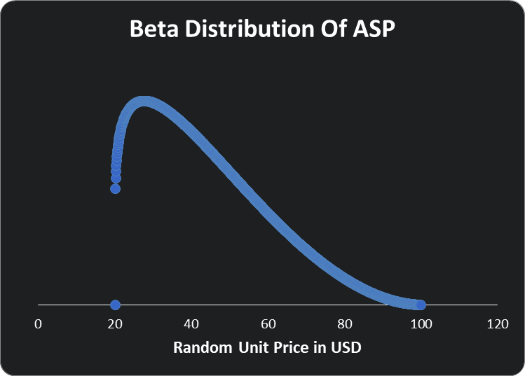
There are lots of ways to add various distributions in Excel. Normal distributions are a good way to start but other distributions, random samplings, or other methods can help reflect our understanding and provide more realistic predictions.

Additionally, our sales department does say that if our competitor beats us in getting to the market first we will have to sell at our lowest ASP. Our market research indicates there is only a 30% chance of that happening based on all of our previous product releases. 

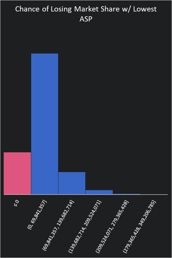
Now we have a 20% chance of losing money. Our ranges haven’t changed and neither have our estimates but we are adding insight into our model. 

Our manufacturing has noticed an issue. It won’t have all year to manufacture because some of this year will be taken up by the development of the product itself. Our finance highlights that we are also not taking into account 2 huge things:

1. The time value of money.

2. If our margins aren’t above 30% we should invest elsewhere as we could get a better return. 

This substantially changes our model. We need to reduce the amount of product produced by the time it takes to develop and discount our profit based on the time it takes to get to market.

Additionally, we have to call the project a failure if we don’t hit a margin of 30%. Our new distribution of possible outcomes looks like this. 

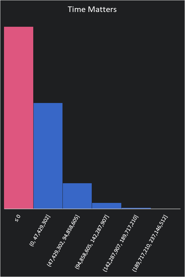
We either lose money or had better opportunities in 70% of our simulations. Our midpoint average has not changed. We still think we should make $53.5 Million but the negative scenarios are extreme and we could lose up to $152 Million. We also have a pretty high chance of failing.

Mitigating Risk:

The team gets together to try and mitigate the risk of the project. The first attempt is to reduce development costs. The team indicates that they can cut the costs to only $300,000 a week if we outsource the project. Though our experience indicates that may double the time it takes to release our product. All things being equal that makes things worse: 

With our cheap outsourcing provider, we now lose 87.6% of the time. What if we got more experts in our company to swarm the project and speed things up? 

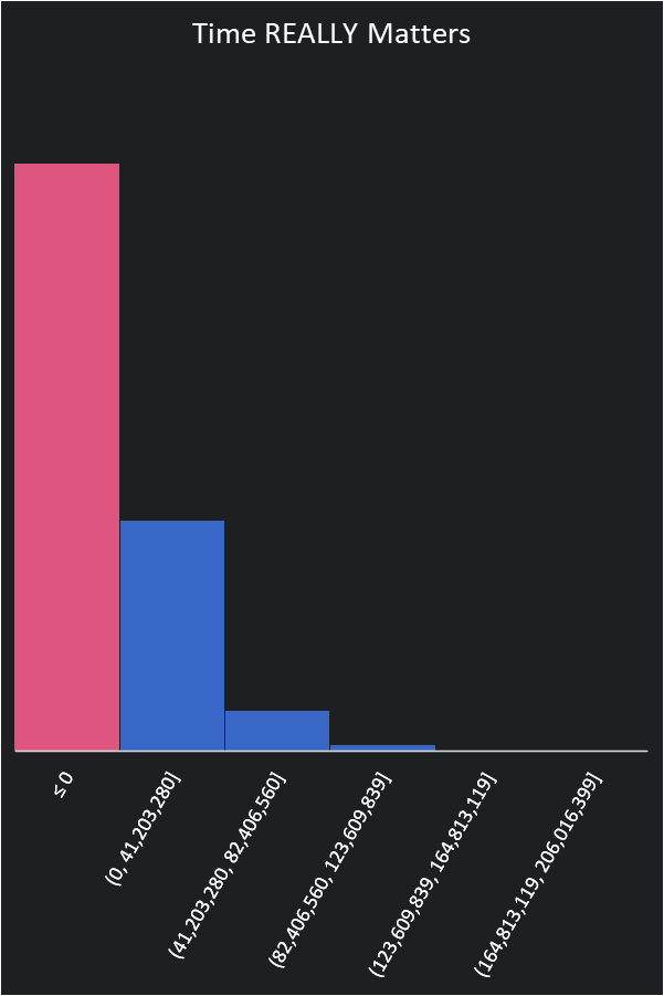
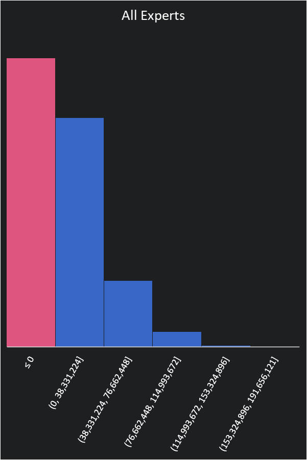
It looks like this is possible, and while it would cost us $3 million a week they estimate they could be done in half the time. Manufacturing indicates if they put their experts in the mix they can probably find a way to better manufacture the parts but they’ll need to work with the dev team. Getting all the experts together increases our dev costs to 3.5 million weekly. The margin risk is our biggest financial risk so getting that off the table helps quite a bit. We now are successful 50% of the time. 

Research has shown that the number one predictor of return on investment is user demand for a product. By focusing on user market research and demand, the marketing team thinks they can tighten the range to 350-500k a month then our prospects of making a profit get much better. 

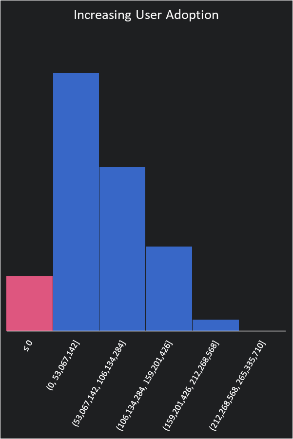
Our chance to succeed is now 86% but it will take some work to get there. We could continue and see what it would look like for manufacturing to work with the dev team to increase production to meet demand. 

The key here is we never changed the estimate ranges but we grew our understanding. We identified risk and added it to the model. When we visualized it that helped us make more informed decisions. If we hadn’t and just gone with the averages we had initially we may have lost a lot of money and not known why our outcome didn’t meet our initial projections. 

Final Thoughts:

One of the main benefits of this process is gaining a mutual understanding. If you aren’t bringing all the different participants to the table then you end up with limited understanding, and what may be worse is groups that are left out won’t buy-in on the outcomes. Consider leaving manufacturing out of the conversation. They wouldn’t understand how critical increasing the production may be to the overall success and as a result more pushback and delay. 

Omitted from this article is how we got to this meeting. There is a process I prefer doing before this called: assumption mapping. Where you try and map out the 3 main risks to a project: do people want it (desirability), can we do it (feasibility), and will we make money doing it (viability)? I will cover more on this process in a future article. 

A Monte Carlo simulator is a viability tester. However, we have to feed in desirability and feasibility estimates to the simulation or it doesn’t work. As we saw and have stated over and over on this site, desirability is the number one predictor of success. We know this to be intuitively true, as we can make cheap boxes with dirt but unless someone really wants them we are wasting our time. 

Charles Lambdin created an excellent article on the cost of delay estimation. It is he does a great job of summarizing Hubbard’s estimation technique outlined in his book, How to Measure Anything: Finding the Value of Intangibles in Business 3rd Edition
by Douglas W. Hubbard (Author)